Category: General

My 2019-era Dell laptop died recently, a few days after I’d replaced the battery. More specifically, the laptop was still running fine off the battery but it had lost its ability to charge from the mains. Without any way to recharge the battery, the laptop was useless.

The green LED on the charger would just turn off when I plugged it into laptop, and the laptop did not detect a charger. The charger itself was fine – I measured the expected 19.5v when the green LED was on, but 0v after plugging it into the laptop. This was clearly bad news, but with a small glimmer of hope. The charger was clearly detecting a short and shutting down (nice safety measure). Perhaps it was just the laptop power jack that was shorted? Unfortunately not – I opened up the laptop, removed the jack and its motherboard cable and that part wasn’t shorted. I could even put the liberated jack/cable assembly onto the power supply and the green LED happily stayed on.

The short was clearly on the motherboard itself – quickly confirmed with a continuity check on the motherboard connector – 0.2ohms. However, the fact that the laptop ran off the battery meant that the fault must be isolated to the charging section only – another glimmer of hope.

Fortunately, the badcaps website had both a circuit diagram and a CAD/layout file for my laptop model.

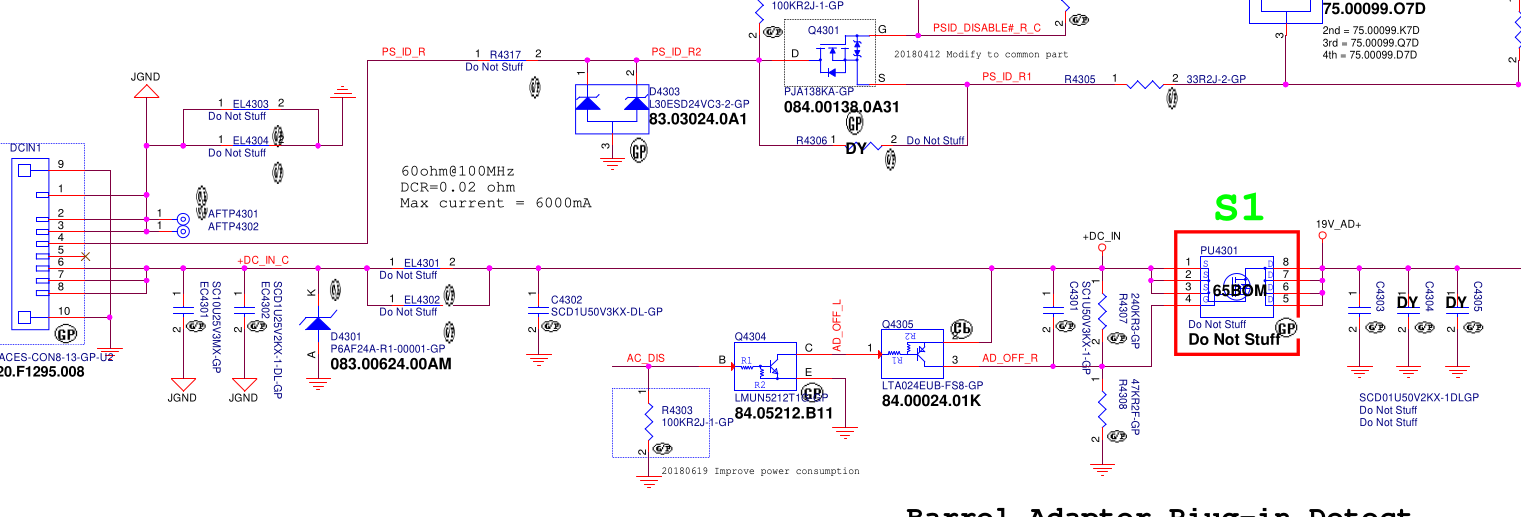
On the left is the power connector, with grounds at the top and power at the bottom. The 19.5v rail has a 10uF cap smoothing cap, a couple of 1uF’s and a zener diode to stabilize the voltage. This is all pretty vanilla so far. Next there’s a big mosfet switch, whose gate is controlled by some ‘AC DISABLE’ line. But crucially, this mosfet helped narrow down the fault since it’s open when the laptop is powered down. Prodding around with the continuity meter showed that everything to the left of the mosfet was shorted, whereas everything on the right was fine. So now we’ve narrowed the suspects down to 3 caps and 1 zener diode. If I had to bet, I’d guess it would be the 10uF cap, since 10uF is a lot of capacitance to fit into a tiny 0603 ceramic cap and must require lots of super-thin dielectric layers. But we need more than a guess.

The badcaps site also had a .cad file. What format is .cad? Fortunately it was a simple textual format containing a comment “USER MENTOR GRAPHICS” which was enough to identify it as GenCad format. And happily the latest version of OpenBoardViewer can read GenCad and display the layout. (It’s a 2 sided board, and it took me a while to realise that hitting spacebar flips to show the other side!).

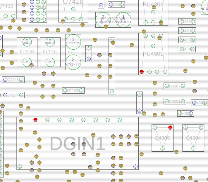
This shows the power connector (DCIN1), and the 10uF cap just above it (EC4301).

How to tell which component has shorted? If all the current is going through a shorted cap, it should be getting hot. I have a current-limited bench PSU, so I set it to max 1A, hooked up ground and then .. very carefully .. used a sharp multimeter probe to apply 1V to the right hand pins of the DCIN connector (this rail normally gets 19.5v so 1v is safe). As expected, the current limiter kicked in. I left it powered up for a few seconds, then used my finger to check if any of the caps or diodes were hot – but nothing obvious.

Next, I tried a more sensitive method – spread some isopropyl alcohol to wet all the nearby components, power up the circuit, and watch carefully to see if the IPA evaporates quickly from any one place. First few attempts were flops, then eventually I built up the courage to send 2A and then 3A through the board. At 3A, it became clear that the 10uF cap and the circuit board near it was drying up quickly, whereas the zeners and mosfets stayed wet. Success – we’ve identified which component is shorted! (an IR camera would’ve also been useful, but they’re pricey and I don’t have one).

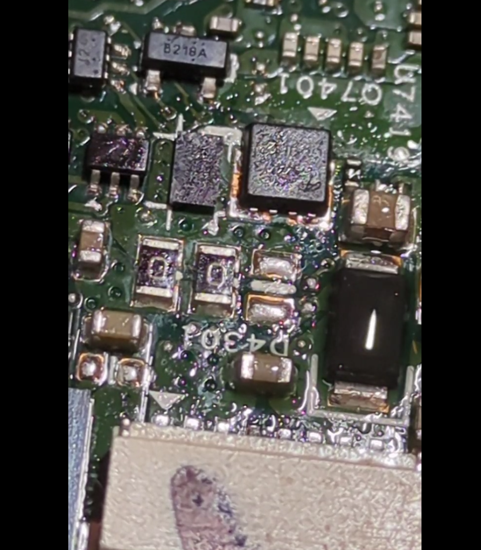
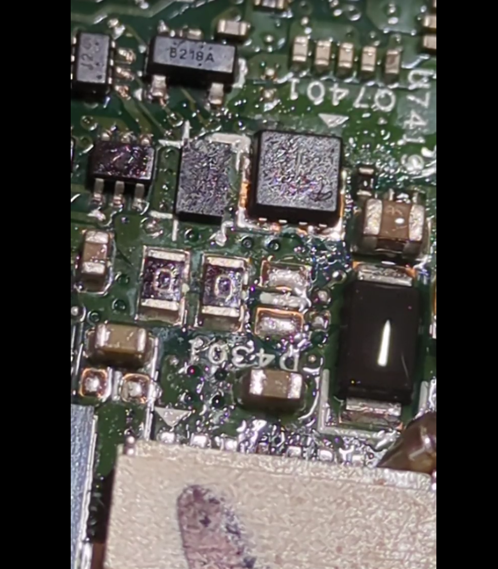
(In the left/before photo, the brown cap in the bottom-middle and the black zener diode are wet. In the right/after photo, the brown cap has dried whereas the black zener is still wet).

Up to this point, I have done SMD soldering exactly once in my life – building a ‘practice kit’ where you soldered 50 tiny SMD resistors to make a dummy load of radio testing. So the idea of trying to remove this failed 10uF from a laptop was somewhat scary. It’s 1.5mm long, and next to lots of even smaller components. But I figured there was a 50/50 chance of success, and so it was rational to ‘invest’ up to 50% of the value of the laptop in tooling (!) and so I acquired a hot-air rework station.

Being keenly aware that any mistake would fry the laptop, I also bought a couple of cheap “SMD practice kits” where you solder some 555s and decade counters and a heap of resistors, diodes, LEDs and transistors to make a pointless flashy light thing. After a few evenings practising, I felt like I had figured out the right temperature + airflow settings, as well as how to use solder paste and tweezers and magnification. When the hot-air works, it’s amazing – the solder melts and surface tensions pulls the component neatly into position. But I also learned to loathe SMD 1N4148 diodes, which are cylindrical and inevitably roll away, arg. The practice kit also says (in Chinese) that some components are deliberately defective, in order to let you “practice debugging as well as soldering”. I suspect ALL the components are rejects, and the fact that any of them worked is a miracle. In the end, the 4017 counter was fried but everything else worked. I desoldered and resoldered the 4017 several times to debug the problem, which was just more useful practice. In the end, 375C and 10% flow works well for soldering, but desoldering needs 30-40% flow so you can get one component hot quickly.

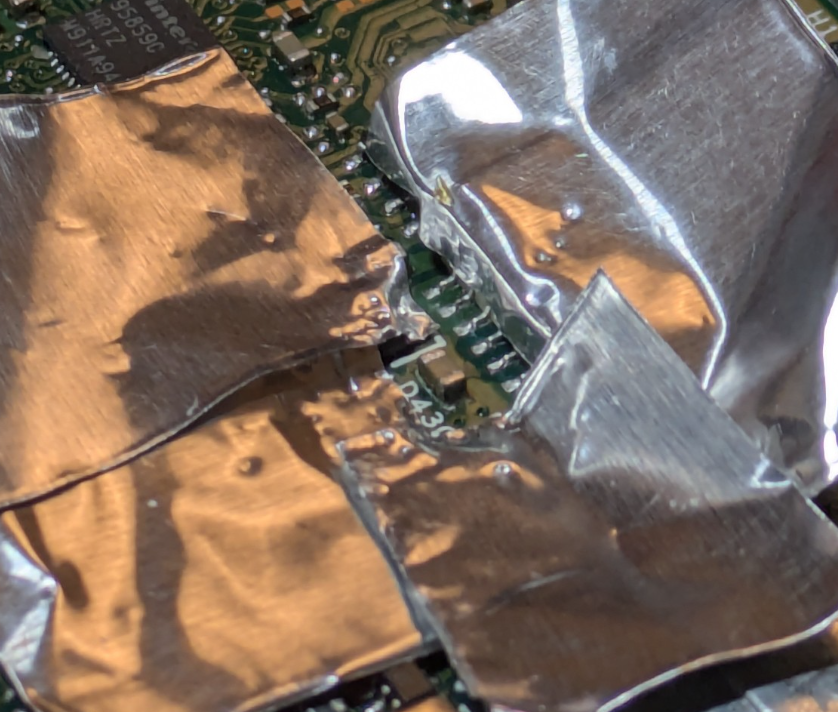
Youtube is amazing for learning new skills – this video in particular highlighted the value of using aluminium tape as temporary heat shielding, a brilliant idea. Most youtubers use pricey digital microscopes when working on SMDs. I mostly made do with cheap jewelers loupes, but at one point I was taking photos of the motherboard and I realised my phone (pixel 7a) was capable of acting as a digital microscope. I reused a camera clamp mount I already had, and hey presto – instant digital microscope for no additional outlay!

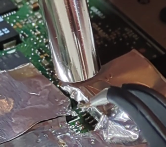
Finally, it was time for laptop surgery. I used the aluminium tape to isolate the failed cap – protecting the plastic power connector and covering nearby SMD components to try and stop them melting + blowing away.

Then I applied flux, held the cap with tweezers and applied heat and … nothing happened.

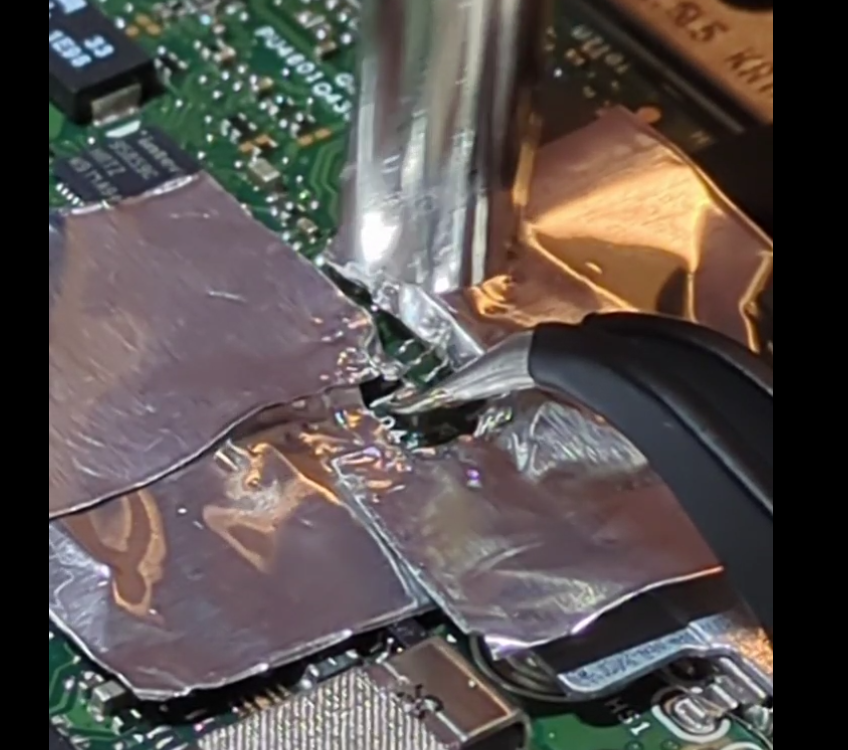
The cap felt like it was glued down. I tried again, keeping the heat on for much longer than I’d ever needed before. Still no movement. I tried increasing the temperate and airflow from 350 to 375C. Still no joy. Maybe the cap really was glued down? Maybe when it shorted it somehow stuck itself to the motherboard?

I tried switching back to my fine-tipped soldering iron, switching from one side to the other to try and get both sides molten and perhaps flick it out of position. Again, no joy. Then I remembered another youtube tip of adding some extra (leaded) solder to hopefully reduce the melting point of the existing likely lead-free stuff. But it still wouldn’t shift.

This was completely unlike the practice boards. On the practice boards, the components heated up quickly, the solder very visibly melted and it was easy to lift them off with tweezers. What could be different? I realised that the answer is that the laptop has a huuge ground plane – and all that mass of copper was just sucking the heat away quickly.

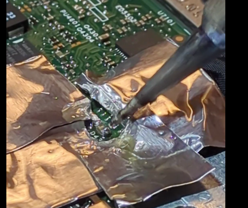
Nothing ventured, nothing gained .. so I turned up the temperature to 400C and 30% air, added more flux, and heated. And heated. And heated. And then – miracle of miracles, the solder melted and the capacitor lifted free!

After a week and a half of build up, this was the mugshot:

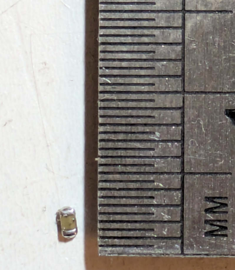
All that work for a 1.5mm long 0603 10uF capacitor. Resistance: 0 ohms. More of a “conductor” than a capacitor.

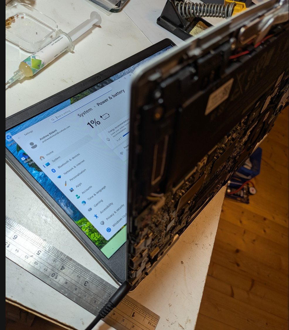
A quick check with the multimeter showed that the power line was no longer shorted. The mains charger kept its green LED of happiness on, and the laptop battery went from 0% charge to 1% charge quickly. Success!!

So all that remains is to get a replacement 10uF 25V capacitor and solder it in. The laptop works fine without it, at least in the short term. Internally, the 19.5v just gets stepped down to 12v, 5v, 3.3v etc anyway. But the designers presumably want the incoming power to be as smooth as possible, so I replaced it like-for-like.

Preparing the pads for the new capacitor was an adventure.  I initially tried cleaning the pads with solder braid and my soldering iron’s finest tip.  But the soldering iron just stuck itself to the board!  I quickly realised that the big ground plane was winning a tug’o’war with my 25W soldering iron, sucking all the heat away and causing the solder at the tip to solidify!  Switching to the biggest tip solved the problem, although now it was super fiddly to manoeuvre the iron into place without bumping other components.

Soldering the cap into place was similar to the desoldering operation.  Aluminium foil everywhere!  I added a bit too much solder paste which balled up on the pads.  I initially held the new capacitor with tweezers in the molten solder and let it cool.  However, the cap ended up looking “high up” on the board.  A second pass just using hot air at 20% flow remelted the solder, and the capacitor sunk down and nicely aligned itself.

A continuity check showed that we had a clean connection to ground on one side, and to the power rail on the other end.  I had also measured the capacitance between ground + power beforehand at 0.17uF, and this went up to 3.9uF with the new cap.   I was expecting 2uF before and 12uF afterwards, but I suppose the zener diode or other components might be messing with my capacitance readings?  Regardless, there was a clear increase in capacitance which gave me confidence that the new capacitor was working.

A successful outcome!  One laptop saved. 

For variety, I switched from SageMath to Sympy since Sympy is a small more focused package. However, I’m struggling with it’s lack of seeming lack of equational reasoning. When you define an equation via Eq(lhs,rhs), it’s not a “first class” object – ie. you can’t divide it by 2 and expect both sides to be half as big, and you have to manually say “subs(titute) eq.lhs with eq.rhs” each time. Finally, I haven’t found good ways to say “substitute just this one occurrence of foo” – sympy wants to do them all. This is all totally anathema to how I think about maths – I’m used to pointing at some subexpression and saying “and use equation 2 to simplify that” etc.

To try out Sympy, I took up the challenge in Chapter 1 of Nahin’s Transients or Electrical Engineers book, in which he conjures up a second-order differential equation for a simple R/L/C ciruit and invites the reader to check he’s not lying. This was a decent workout, since 1) it involves first- and second-derivatives, 2) it involves plenty of equations and manipulating expressions. To be honest, I found this hard. I tried doing it on computer and got nowhere. I then did it by hand using paper and pen to figure out the steps. Then I went back to the computer and had to tackle several “how do I get the computer to do x” puzzles before I got anywhere.

In the end, I did indeed verify that Nahin is telling the truth (phew!) but it was hours and hour of headscratching work. It’s nice to have the computer verify I haven’t err’d in my derivation, but this was not “computer makes task easier” stuff – quite the opposite! I guess the nice bit comes later when I can get the computer to actually solve the differential equations for concrete cases. But this ‘abstract algebra manipulation’ stuff is painful.

In the end, the “proof” looks like..

from sympy import *
from sympy.abc import R,L,C,t

i = Function("i")(t)
i1 = Function("i1")(t)
i2 = Function("i2")(t)
v = Function("v")(t)
u = Function("u")(t)

# Chapter 1 of Transients For Electrical Engineers

# Equations which describe the given "R ser L par (R ser C)" circuit (ie. KVL/KCL)
eq1 = Eq(i, i1 + i2 )
eq2 = Eq(u, i*R + v)
eq3 = Eq(v, L * i1.diff())
eq4 = Eq(v, i2*R + (1/C) * Integral(i2,(t,0,t)))

# The book states a large differential equation with 'input' voltage u(t) + derivative on left,
# and current i(t) (+derivatives) on right
(u.diff(t,2) + (R/L) * u.diff() + 1/(L*C)*u)

# and challenges you to check the equality does actually follow from above 4 equations

# First step is easy; there's only one equation involving 'u' so let's apply that everywhere
_.subs( eq2.lhs, eq2.rhs).simplify()

# Now we have to be tactical; we have v and v' and v'' but we want to do different things to each
# I don't know how to tell sympy to "just substitutes the first instance, not all instances"
# So start by substituting for v'' (since that leaves v' and v alone for now) and use eq4 the capacitor eqn
_.subs(eq4.lhs.diff(t,2), eq4.rhs.diff(t,2)).simplify()

# And now we can tackle v' and then v - both use eq3 (the inductor one)
# This leaves us with just currents, albeit a mixture of i/i1/i2
_.subs(eq3.lhs.diff(t), eq3.rhs.diff(t)).simplify()
_.subs(eq3.lhs,eq3.rhs).expand().simplify()

# Now we want to group + collapse the i1's and i2's using eq1.
# But I don't know how to get sympy to "see" that we have lots of (i1+i2) patterns 
# So as a hack, we can always subtract something then add something equal to it and preserve equality, right?
# So we use that to turn i1+i2 into i ...
(_ + diff(eq1.rewrite(Add),t)/C).expand()

# Getting there .. now we need to sweep up the twice-differentiated cases..
(_ + R*eq1.rewrite(Add).diff(t,2)).expand()
# w^5 - which was what we wanted

Using Sagemath for electronics is nice because it forces you to be explicit about your assumptions and calculations. Ideally, you’d start by telling Sagemath about Maxwell’s laws and build up from there. For DC conditions, like calculating the bias for a common emitter amplifier we can assume no changing magnetic fields, so Faraday’s law of induction simplifies to Kirchhoff’s Voltage Law. We also need Ohm’s Law for the voltage-current relationship in resistors. I supplied the series/parallel resistance formula (but those too could come from KVL/KCL + Ohms law).

First let’s tell Sagemath about Kirchhoff’s Voltage Law:

from functools import reduce
from operator import add, neg

# Teach sagemath about physics (Faraday's law of induction in its KVL guise)

# Kirchhoff voltage law says sum of voltage drops around a loop is zero.
# Note: this is really just Faraday's law of inducion, for the special case of no changing magnetic fields
# Note: this is taking in symbolic expressions, and returning a symbolic expression
def KVL( voltages ): 
    return reduce(add,voltages) == 0

# Convenience case for where we have one voltage source, then we give remaining voltage drops as positive values 
# ie. KVL_vsource(5, [1,2,x] means a 5v source, then drop of 1v then drop of 2v then drop of x volts.
def KVL_vsource( vsource, vothers ):
     return KVL( [vsource] + list(map(neg,vothers)))

Next, let’s tell it about series/parallel resistors and Thevenin equivalent for voltage dividers (again, would be nice to derive this from KVL/KCL/Ohm)

# Kirchhoff's Current Law (aka conservation of charge) and Ohms Law give composition rules for impedance
# TODO: derive directly from KCL/Ohm.
recip(x) = 1 / x
ipar(a,b) = recip( recip(a) + recip(b))
iser(a,b) = a + b

# Thevenin equivalent voltage/resistance for divider (r1 and r2)
Vth_divider(v, r1, r2) = v * r2 / (r1+r2)
Rth_divider(r1, r2) = ipar(r1,r2)

Now we can pick some values for a common-emitter amplifier

# Transistor params
beta = 100
Vbe = 0.7

# Common emitter amplifier, biased using divider, with emitter feedback
Vcc = 5
Rtop,Rbot = 10e3, 3.3e3
Re = 470
Rc = 2e3

And calculate the quiescent voltages + currents:

# Turn the divider into thevenin equivalent
Vth = Vth_divider(Vcc, Rtop, Rbot )
Rth = Rth_divider(Rtop, Rbot)

# To get Ib, we use Kirchhoff's Voltage Law for loop around base/emitter, and solve for Ib
Ib = var("Ib")
eqn = KVL_vsource( Vth, [ Ib*Rth, Vbe, beta*Ib*Re])
print("KVL equation is ", eqn)
Ib = solve(eqn, Ib, solution_dict=True)[0][Ib].n()
print("So Ib is", Ib*1000, "mA")
# Finally, get voltage drop over Rc to get output voltage.
Ic = beta * Ib

Vc = Vcc - Ic * Rc
print("Vc is ", Vc)

var("Vce")
vce_eqn = KVL_vsource(Vcc, [Ic*Rc, Vce, Ic*Re])
Vce = solve(vce_eqn, Vce, solution_dict=True)[0][Vce].n()
print("Vce is ", Vce)

Here we’re just using Sagemath as a numeric calculator. It’s kinda neat to package up Kirchhoff’s Voltage Law so we can just state all the knowns and let Sagemath find the unknowns, without us having to do algebra. But fundamentally, this is stuff we could easily do in excel/python/etc.

But with Sagemath we can stick with symbolic expression. Let’s start by keeping the potential divider as-is, but we’ll make Rc and Re symbols.

# Common emitter amplifier, biased using divider, with emitter feedback
Vcc = 5
Rtop = 10e3
Rbot = 3.3e3
Re = var("Re")
Rc = var("Rc")

# Turn the divider into thevenin equivalent
# Note: some textbooks just ignore supply impedance, ie. assume it's a perfect voltage source which has fixed voltage
# regardless of how much current is drawn; this isn't the case for resistor-divider.  We can either make heuristic assumptions
# (eg. assume load has "high enough" impedance, so draws little current) or we can calculate exactly via Thevenin equivalent.
Vth = Vth_divider(Vcc, Rtop, Rbot )
Rth = Rth_divider(Rtop, Rbot)

# To get Ib, we use Kirchhoff's Voltage Law for loop around base/emitter, and solve for Ib
Ib = var("Ib")
eqn = KVL_vsource( Vth, [ Ib*Rth, Vbe, beta*Ib*Re])
Ib = solve(eqn, Ib, solution_dict=True)[0][Ib]
Ic = beta * Ib

Vc = Vcc - Ic * Rc
print("Vc is ", Vc)
solve([Vc == Vcc/2, Ic*Re==Vcc/10], [Rc,Re], solution_dict=True)

# Output:
Vc is  -719/10*Rc/(133*Re + 3300) + 5

So now the collector voltage is left as an expression, dependent on the (as yet unchosen values of Rc and Re).

Rather than picking them manually, we can express constraints:

solve([Vc == Vcc/2, Ic*Re==Vcc/10], [Rc,Re], solution_dict=True

# Output
[{Rc: 13750/9, Re: 2750/9}]

So we’ve effectively just stated the design rules of “collector should be midrail” and “Ve should be about 10% of supply”, and Sagemath has found the values of Rc and Re which “make it so”. Nice.

How about if we wanted IC=20mA and Vc at midrail?

solve([Vc == Vcc/2,  Ic==0.01], [Rc,Re], solution_dict=True)

# Output
[{Rc: 250, Re: 3890/133}]

This time we used Sagemath to model an LC bandpass filter, centered on 100MHz, and calculate the insertion loss in dB at various frequencies. It’s based on what the filter calculator defaults to for a 1st order shunt-first Chebyshev bandpass filter.

# Complex impedance for capacitor and inductor
C(c,f) = -I / (2 * pi * f * c)
L(l,f) = I * 2 * pi * f * l

# Composition rules for impedance
recip(x) = 1 / x
ipar2(a,b) = recip( recip(a) + recip(b))
ipar3(a,b,c) = recip( recip(a) + recip(b) + recip(c))
iser(a,b) = a + b

# A simple RC lowpass filter
V = 10
Rs = 50 # source impedance
Rl = 50 # load impedance

# These are just the default values from https://rf-tools.com/lc-filter/
# They give a bandpass filter centered at 100MHz, with 20MHz bandwidth.
C1 = 48.58e-12
L1 = 52.67e-9

# This is the overall LC bandpass filter, with source impedance and load.
impedance = iser( Rs, ipar3(C(C1,f),L(L1,f),Rl) )

# The filter website shows insertion loss, which looks at how the power in the load
# is affected by putting in the LC filter.

power(v,r) = (v^2 / r).abs()

# Without our filter ("device under test"), the power is simple - half the voltage
# is dropped over the source impedance, leaving half for the load.
power_without_dut = power(V/2,Rl)

# To calculate power in load with our filter, we need to know the current
current = V / impedance
V_over_load = V - (current * Rs)
power_in_load = power(V_over_load, Rl)

as_dB(frac) = log(frac,10) * 10
insertion_loss_dB = as_dB(power_in_load / power_without_dut)

insertion_loss_dB(51750194).n()  # ans: -3.29183565814456
insertion_loss_dB(41896869).n()  # ans: -5.05202056128256

These values for insertion loss match what the calculator website shows in the “S parameters” tab.

How to think about this? If you take away the LC bit, you’re just left with a “maximum power theorem” situation, ie. source impedance and load impedance are both constant and equal.

Now, let’s introduce the LC again but imagine that there’s some magic circumstance in which it’s impedance ends up zero – meaning we’ll still be in “maximum power theorem” situation. Since the L and C are of “opposite nature”, there’ll be some frequency where the L has reactance-blah reactance at the same time as the C has negative-blah impedance. With the L and C in parallel we sum their impedances (actually, reciprocal of sum of reciprocals) so they cancel out.

In all other circumstances, either the L will “win” with a larger reactance or the C will “win” and we’ll net out to the L-par-C having some non-zero impedance. This will pull us away from our perfect 50ohm “maximum power” point and the power in the load will be less.

At low frequencies, the inductor (L) will present a low-impedance path, meaning that the overall impedance will be much lower than 50. This results in a higher current, a greater voltage drop over the source impedance leaving our parallel RLC bundle seeing a lower voltage.

At high frequencies, it’s the capacitor which presents a low-impedance path, and by the same argument, we get a lower voltage over our load.

But when we’re dealing with RF we’re dealing with waves, and when there’s a change in impedance you get reflections. If our bandpass filter only had 50ohms impedance at it’s centre frequency, then it has a non-50ohm impedance everywhere else – which causes reflections. Actually, this is kinda obvious from conservation of energy: if there’s energy coming in, but it’s not ending up in the load then either it’s absorbed in the filter itself or it must be reflected. If our filter was absorbing energy, it would be heating up (unlikely, since we build filters with low-resistance components), or it would have to be radiating (unlikely unless the filter was physically very big).

If we’re using a bandpass filter at the input of a receiver, all the signals outside the passband are getting bounced back towards the antenna (the amount of energy here is tiny so it’s not a problem).

If we use a lowpass filter to “get rid of” harmonics at the output of a transmitter, the energy of those harmonics is heading straight back towards the power amp.

If we use an IF bandpass filter in a superhet receiver, then those reflected signals will be heading back towards a mixer where they can re-mix and cause problems.

If we’re worried by those reflections, what can we do? The answer is to use a diplexer – essentially a fork in the road leading to a lowpass and highpass filters respectively. Whichever part (low or high frequencies) we don’t want can be sent to a 50ohm terminator to be absorbed and turned into heat – and overall the whole thing looks like 50ohms across all frequencies This is something I’ve seen used in the “High Performance Direct Conversion Receivers” ARRL article. Also in this “Popcorn DC Receiver”, this one and this one.

When learning about amateur radio, there’s loads of discussion about reflections that happen when the impedance of your antenna isn’t 50ohm at the frequency you’re sending on. This leads to reflections back up your 50ohm coax, and the sum of the outgoing and reflected wave leads to standing waves. The standing waves can be characterised by the “standing wave ratio” (SWR) which is a measurable quantity, and can therefore be used to indicate that your antenna impedance isn’t right. However, if your feeder cable is attenuating the waves, the reflected wave might be weak by the time it gets back to the home end of the cable – which could wrongly lead you to infer that you have the impedance spot on.

Despite all this chatter about reflections from the antenna, I have seen almost no mention of reflections from filtering steps. I guess it’s just a question of degree. Reflections from antennas are bad because its potentially the full transmit power at your transmit frequency that’s bouncing back. Your lowpass filter is also after the power amp, but in normal operation the reflected power is much small since it’s only the power from the harmonics that bounces back. If your power amp was very very nonlinear you might have more power in your harmonics. Or if you had been sending at 7MHz with a 8MHz lowpass filter, and then switched up to sending at 14MHz but didn’t change to an appropriate lowpass filter you’d end up getting all your transmit power bouncing back.

I entered this particular rabbithole with a desire to understand how the various kinds of passive filters work. I’ve already physically constructed bandpass and lowpass filters, but I had to get the values for my capacitors and hand-wound inductors from a mysterious but helpful online filter calculator. Being a cynical kinda person, I first “built” each filter using ngspice (the circuit simulation tool) to check they looked sane before heating up my soldering iron.

But that online filter calculator is kinda mysterious. It lets you build various kinds of filters – Butterworth, Chebyshev, Elliptic – and each one comes in different flavours, such as shunt-first or series-first.

They’re all made from combinations of capacitors and inductors – the two standard frequency-dependent building blocks, which harness electric and magnetic fields respectively. I know how a capacitor behaves on its own, and I know how an inductor behaves on its own – but I don’t know what magic happens when you put a bunch of them together.

Buoyed by previous suggest in modelling pi-attenuators in Sagemath from first principles, I decided to go on a journey to also model various families of passive filters in Sagemath too. The hope is that I “tell” Sagemath about the axioms – what the impedance of each component is, and how series/parallel combinations work – along with the combinations of capacitors/inductors that make up a filter, and out should pop the shapes of whatever bandpass filter you like Of course, this is exactly what the SPICE simulator will do. But the attractive thing about Sagemath is that it’s tracking the entire equation relating everything, and hence you can ask many more questions of it.

I initially tried to dive straight in an model a 3rd order Chebyshev bandpass filter. I got kinda close, but couldn’t get to the point of having correct bandpass filter behaviour. So I took that as a hint that perhaps I should be starting with something simpler.

The simplest frequency-dependent circuit is an RC filter. I’ll use R=4700ohm and C=47nF. The resistor (with constant impedance) and capacitor (with impedance that decreases as frequency rises) act as a potential divider.

Now, a RC filter is simple enough that you can work it out by hand directly. Since I use emacs a lot, I often use emacs lisp as a kind of quick calculator, so here’s how I calculate the impedance (xc) and the output voltage (assuming 10v sine input):

(defun 1/ (x) (/ 1 x))
(defun sq (x) (* x x))

(let* ((f 10e3)
       (c 47e-9)
       (r 4700)
       (xc (1/ (* 2 pi f c))))
       (* 10 (/ xc (sqrt (+ (sq r) (sq xc))))))

;; Give 0.719, meaning at 10kHz the output is 0.719 volts.

I can also use ngspice to simulate the circuit, and do a sweep across frequencies:

RC filter

Vin 1 0 DC 0 AC 10
R1 1 2 4700
C1 2 0 47e-9

.control
AC LIN 10000 1 20000
run
set hcopypscolor
hardcopy rc.ps vm(2) xlimit 0 11k
shell evince rc.ps
.endc
.end

This plot visually confirms that at 10kHz, voltages is around 0.7v.

Now for the sagemath attempt. Sagemath knows about complex numbers, so we can represent impedances directly as complex numbers (sagemath uses uppercase I):

# Complex impedance for capacitor and inductor
C(c,f) = -I / (2 * pi * f * c)
L(l,f) = I * 2 * pi * f * l

# Composition rules for impedance
recip(x) = 1 / x
ipar(a,b) = recip( recip(a) + recip(b))
iser(a,b) = a + b

# If you have [v] volts across  a potential divider 
# consisting of impedance [a] on top, [b] below, 
# connected to [load], what voltage does the load see?
pd_vout(v, a, b, load) = v * ipar(b,load) / iser(a,ipar(b,load))

# Our example RC lowpass filter
R1 = 4700
C1 = 47e-9
overall = pd_vout(10, R1, C(C1,f), 10e9)

# What's the voltage at 10kHz?  Note: use n() to get 
# a number instead of a maths expression, and abs() to
# get the complex magnitude
overall(10e3).n().abs()

# Answer: 0.718621364643

It gets the right answer, but what’s interesting (to me) is that it’s clearly there’s no additional magic going on. Spice might be doing all sorts of elaborate things to get it’s answer. But in our Sagemath version, it’s obvious that the only ingredients are 1) impedance, represented as a complex number, 2) combinations of impedances, and 3) ohms law, as expressed in the potential divider equation.

In the next post, I’ll move onto something rather more useful – an LC bandpass filter.