Spice vs Sagemath

I entered this particular rabbithole with a desire to understand how the various kinds of passive filters work. I’ve already physically constructed bandpass and lowpass filters, but I had to get the values for my capacitors and hand-wound inductors from a mysterious but helpful online filter calculator. Being a cynical kinda person, I first “built” each filter using ngspice (the circuit simulation tool) to check they looked sane before heating up my soldering iron.

But that online filter calculator is kinda mysterious. It lets you build various kinds of filters – Butterworth, Chebyshev, Elliptic – and each one comes in different flavours, such as shunt-first or series-first.

They’re all made from combinations of capacitors and inductors – the two standard frequency-dependent building blocks, which harness electric and magnetic fields respectively. I know how a capacitor behaves on its own, and I know how an inductor behaves on its own – but I don’t know what magic happens when you put a bunch of them together.

Buoyed by previous suggest in modelling pi-attenuators in Sagemath from first principles, I decided to go on a journey to also model various families of passive filters in Sagemath too. The hope is that I “tell” Sagemath about the axioms – what the impedance of each component is, and how series/parallel combinations work – along with the combinations of capacitors/inductors that make up a filter, and out should pop the shapes of whatever bandpass filter you like Of course, this is exactly what the SPICE simulator will do. But the attractive thing about Sagemath is that it’s tracking the entire equation relating everything, and hence you can ask many more questions of it.

I initially tried to dive straight in an model a 3rd order Chebyshev bandpass filter. I got kinda close, but couldn’t get to the point of having correct bandpass filter behaviour. So I took that as a hint that perhaps I should be starting with something simpler.

The simplest frequency-dependent circuit is an RC filter. I’ll use R=4700ohm and C=47nF. The resistor (with constant impedance) and capacitor (with impedance that decreases as frequency rises) act as a potential divider.

Now, a RC filter is simple enough that you can work it out by hand directly. Since I use emacs a lot, I often use emacs lisp as a kind of quick calculator, so here’s how I calculate the impedance (xc) and the output voltage (assuming 10v sine input):

(defun 1/ (x) (/ 1 x))
(defun sq (x) (* x x))

(let* ((f 10e3)
       (c 47e-9)
       (r 4700)
       (xc (1/ (* 2 pi f c))))
       (* 10 (/ xc (sqrt (+ (sq r) (sq xc))))))

;; Give 0.719, meaning at 10kHz the output is 0.719 volts.

I can also use ngspice to simulate the circuit, and do a sweep across frequencies:

RC filter

Vin 1 0 DC 0 AC 10
R1 1 2 4700
C1 2 0 47e-9

.control
AC LIN 10000 1 20000
run
set hcopypscolor
hardcopy rc.ps vm(2) xlimit 0 11k
shell evince rc.ps
.endc
.end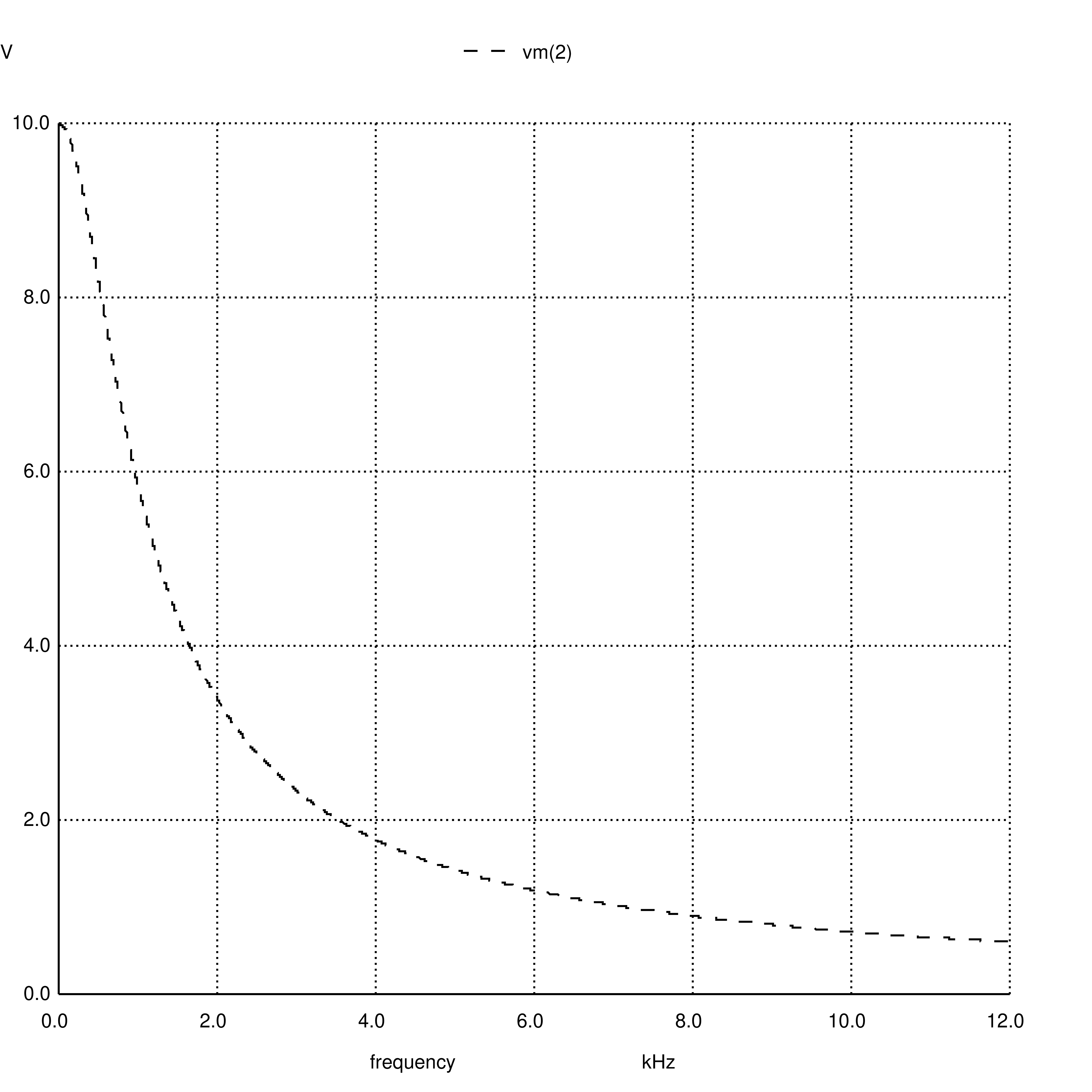

This plot visually confirms that at 10kHz, voltages is around 0.7v.

Now for the sagemath attempt. Sagemath knows about complex numbers, so we can represent impedances directly as complex numbers (sagemath uses uppercase I):

# Complex impedance for capacitor and inductor
C(c,f) = -I / (2 * pi * f * c)
L(l,f) = I * 2 * pi * f * l

# Composition rules for impedance
recip(x) = 1 / x
ipar(a,b) = recip( recip(a) + recip(b))
iser(a,b) = a + b

# If you have [v] volts across  a potential divider 
# consisting of impedance [a] on top, [b] below, 
# connected to [load], what voltage does the load see?
pd_vout(v, a, b, load) = v * ipar(b,load) / iser(a,ipar(b,load))

# Our example RC lowpass filter
R1 = 4700
C1 = 47e-9
overall = pd_vout(10, R1, C(C1,f), 10e9)

# What's the voltage at 10kHz?  Note: use n() to get 
# a number instead of a maths expression, and abs() to
# get the complex magnitude
overall(10e3).n().abs()

# Answer: 0.718621364643

It gets the right answer, but what’s interesting (to me) is that it’s clearly there’s no additional magic going on. Spice might be doing all sorts of elaborate things to get it’s answer. But in our Sagemath version, it’s obvious that the only ingredients are 1) impedance, represented as a complex number, 2) combinations of impedances, and 3) ohms law, as expressed in the potential divider equation.

In the next post, I’ll move onto something rather more useful – an LC bandpass filter.